by
by Samuel Cochran, Brian Gaudette, Jared Myers, and Colton Schang
We started class by discussing descriptive statistics, which are summary statistics (summary of a set of observations) that quantitatively describes/summarizes a collection of data. Professor Markowitz informed us that descriptive statistics need variables and that different types of variables convey different types of information. He then broke down descriptive statistics into its three components:
Nominal: nominal data separate people/things into different categories. These categories are not ordered, one is not “more” or “less” than another. These data are definitive. Examples of nominal data include age, gender, political party, job billet, military rank, school grades, hair color, etc.
Ordinal: ordinal data have natural, ordered categories where the variables are ranked along a scale. These data can tell us that an attribute is “more” or “less” than another, but you cannot say exactly how much more or how much less. Ordinal data are typically measures of non-numeric concepts like satisfaction, happiness, comfort, etc. A popular example is the Likert scale, which you have most often been exposed to when taking surveys. For example, a question may look like this:
Identify which of the following best describes how much you like J580
| Love it! | I like it | Its ok | Don’t like it | Hate it! |
| 1 | 2 | 3 | 4 | 5 |
Interval: Interval data is data that communicates an exact difference. It is also measured along a scale, but it is much more precise. Not only does it tell us the exact difference, but it tells us the order of values as well. For a particular relationship, we can say exactly how much more or less. This data type always appears as numerical values where the distance between the two points is standardized. Interval data is nice because from it we can observe central tendency; from it we can determine the mean, median, mode, and even the standard deviation of a data set. Time is a good example of interval data, because the increments are known, measurable, and consistent.
Professor Markowitz then gave us a hint: For our final project, most of our data will be nominal and ordinal.
During the middle part of class we broached the topic of correlation… Professor Markowitz ran us through a brief history of the Pearson Correlation Coefficient and how Karl Pearson was trying to find a measurement between two variables.

He stressed the importance of the relationship of variables with a positive and negative correlation, between 1 and -1 respectively. We were able to learn that a strong positive relationship means that both variables move together in the same direction, whereas a strong negative relationship moves in the inverse. An example being, if you have a strong positive relationship between the two variable X (Prejudice against non-white people) and Y (Support for Immigration) than that would mean the more prejudice you are against non-white people, you are more likely to support immigration.
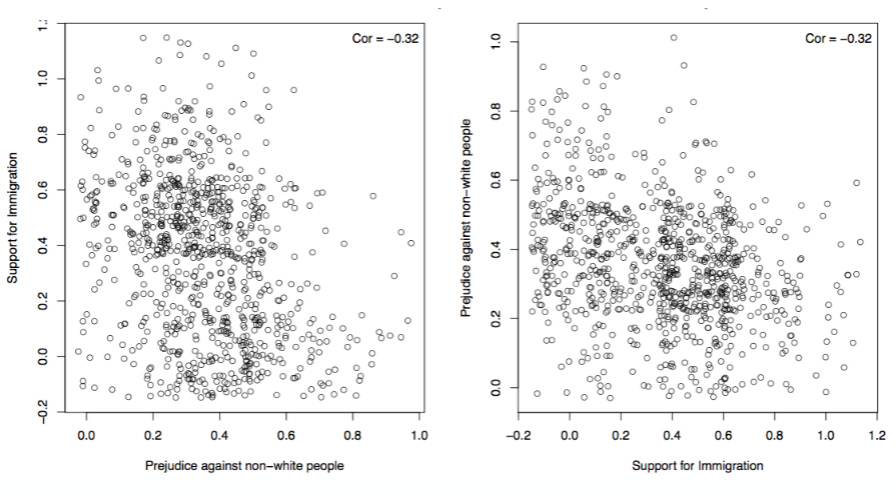
In the charts above, we see that these two variables actually exhibit a NEGATIVE (or inverse) correlation. In other words, more prejudice against non-white people is closely related to lower support for immigration. Note that flipping the X and Y variables does not change the relationship: the correlation value remains the same.
Professor Markowitz reminded us that correlation does not equal causation and that we should always keep that in mind when analyzing two variable and our hypothesis. Take, for example, a less controversial subject: firemen and fires. One could observe a set of data about fires and create a correlation between two pieces of data: the dollar value of damage of a fire and the number of firemen responding to the scene. One could probably assume that the more damaging the fire, the more firemen were there, representing a positive correlation.
What hypotheses could be made from noting this positive correlation? Are firemen causing the fires? Do firemen have some sick fascination that
draw them to a disaster scene for entertainment? Do firemen respond to fires with more presence
the richer the person or business is at the scene? Probably not.
In this case, we would probably find that a third factor is at play,
which would also have a strong positive correlation – the size of the fire.

So, what causes what? By removing the number of firefighters and correlating fire damage and fire size, we could understand how those two variables interact. The same goes for fire damage and number of firefighters. We might even see, upon further inspection, that there are instances of huge fires with high damages where few firemen responded. We might discover that the size of the fire causes more damage and therefore more people are needed to suppress the flames. While correlation provides us clues toward how variables interact with each other, it is far from the whole story.